Advanced R - Hadley Wickham Chapter 17 Big Picture

class: center, middle, inverse, title-slide

# Advanced R - Hadley Wickham <br> Chapter 17 Big Picture
## R Ladies Netherlands Boookclub
### Janine Khuc, October 13, 2020

---

<div>
<style type="text/css">.xaringan-extra-logo {
width: 50px;
height: 128px;
z-index: 0;
background-image: url(R-LadiesGlobal.png);
background-size: contain;
background-repeat: no-repeat;
position: absolute;
top:1em;right:1em;
}
</style>
<script>(function () {
  let tries = 0
  function addLogo () {
    if (typeof slideshow === 'undefined') {
      tries += 1
      if (tries < 10) {
        setTimeout(addLogo, 100)
      }
    } else {
      document.querySelectorAll('.remark-slide-content:not(.title-slide):not(.inverse):not(.hide_logo)')
        .forEach(function (slide) {
          const logo = document.createElement('div')
          logo.classList = 'xaringan-extra-logo'
          logo.href = null
          slide.appendChild(logo)
        })
    }
  }
  document.addEventListener('DOMContentLoaded', addLogo)
})()</script>
</div>

# Welcome!

- This is joint effort between RLadies Nijmegen, Rotterdam,'s-Hertogenbosch (Den Bosch), Amsterdam and Utrecht 
- We meet every 2 weeks to go through a chapter 
--

- There are still possibilities to present a chapter :) Sign up at https://rladiesnl.github.io/book_club/  
- https://advanced-r-solutions.rbind.io/ has some answers and we could PR the ones missing  
- The R4DS book club repo has a Q&A section.https://github.com/r4ds/bookclub-Advanced_R

---
# Introduction
- **Metaprogramming**: modifying the blueprints of computations or programming the program
--

- today we'll focus on a **big picture of metaprogramming**
  - lots of vocabulary will be introduced
  - Chapter 18-21 will introduce the big ideas in more detail
  - a more practical intro to [tidy evaluation](https://tidyeval.tidyverse.org/) covering many concepts
--

- **Disclaimer**: you might be frustrated/ confused at first- and it's the natural process that will happen- so don't worry main thing is to stay curious and ask questions! :)
--

---
# Do you need metaprogramming?
well it depends....

let's assume the following function to do a scatter plot

```r
ggplot(starwars, 
       aes(mass, height)) +
geom_point()
```

---
# Do you need metaprogramming?
If we wanted to reuse the function, we could rewrite it like this:

```r
plot_scatter <- function(data, x_col, y_col) {
  ggplot(data, 
       aes(x_col, y_col)) +
geom_point()
}
```
--

let's try it on the `mtcars` dataset.

```r
plot_scatter(mtcars, disp, mpg)
#> Error in FUN(X[[i]], ...) : object 'disp' not found
```

---
# Do you need metaprogramming?
Does not work. What if we try this?

```r
plot_scatter(mtcars, 'disp', 'mpg')
```

<img src="Ch17_Xaringan_files/figure-html/unnamed-chunk-4-1.png" width="432" style="display: block; margin: auto;" />
--
That's a plot, but not the one we wanted.

---
# Do you need metaprogramming?
And what if we try this?

```r
plot_scatter(mtcars, mtcars$disp, mtcars$mpg)
#> Error: Aesthetics must be either length 1 or the same as the data (87): x and y
```
Still not working...
--

<center>
<img src="https://media.giphy.com/media/DzIIiyZvSdzxu/giphy.gif" width="350" />
</center>
--

Don't you worry! We'll be working towards a solution!

---
# Metaprogramming _can_ be useful!

Metaprogramming is useful to understand this kind of issues, where

-  you'd like to understand some of it to be able to use dataframes in full scope, where column names are named objects 
--

- To translate and execute `R` in a foreign environment e.g. dbplyr
--

- To execute `R` with a more performant compiled language
--

### ideas we'll tackle
1. Code is data
2. Code is a tree
3. Code can generate code
4. Evaluation runs code
5. Customising evaluation with functions
6. Customising evaluation with data
7. Quosures

---
# 1. code is data
- You can capture code and compute on as you can with any type of data
--

- **Expressions**= captured code; and can be captured with `rlang::expr()`
--

```r
expr(mean(x, na.rm = TRUE))
#> mean(x, na.rm = TRUE)
expr(10 + 100 + 1000)
#> 10 + 100 + 1000
```
`expr()` let's you capture code you typed.

---
# Key 1: code is data
Wrapping it into a function.

```r
capture_it <- function(x) {
  expr(x)
}
capture_it(a + b + c)
#> x
```
--

The expression was not captured. We need a different tool to capture code passed to a function. Use `enexpr()` - take "en" as for enriched

```r
capture_it <- function(x) {
  enexpr(x)
}
capture_it(a + b + c)
#> a + b + c
```
because `capture_it()` uses `enexpr`, we say that it automatically **quotes** its first argument. `expr()` captures exactly what it gets, while `enexpr()` passes on what the user inputs.

---
# Key 1: code is data
Once captured, you can inspect and modify it- behaves much like a *list* and can be modified by using `[[` and `$`

```r
f <- expr(f(x = 1, y = 2))
f
#>f(x = 1, y = 2)

# Add a new argument
f$z <- 3
f
#> f(x = 1, y = 2, z = 3)

# Or remove an argument:
f[[2]] <- NULL
f
#> f(y = 2, z = 3)
```

---
# 2. Code is a tree
- Almost every programming language represents code as a tree **abstract syntax tree**
- `R` is special as this tree can be _inspected_ and _manipulated_ once captured.
--

![Source: modified from Hadley Wickham's Tidy evaluation in 5 mins](images/code_as_tree_1.png)

---
## R- code as a tree
![Source: modified from Hadley Wickham's Tidy evaluation in 5 mins](images/code_as_tree_2.png)

---

## More complex calls have multiple levels
![Source: modified from Hadley Wickham's Tidy evaluation in 5 mins](images/code_as_tree_3.png)

---
## More complex calls have multiple levels
![Source: modified from Hadley Wickham's Tidy evaluation in 5 mins](images/code_as_tree_4.png)

---
## Every expression has a tree
![Source: modified from Hadley Wickham's Tidy evaluation in 5 mins](images/code_as_tree_5.png)

---
## Every expression has a tree
![Source: modified from Hadley Wickham's Tidy evaluation in 5 mins](images/code_as_tree_6.png)

---
# R- code as a tree
- R also has a very handy function to display this you can use `lobstr::ast()`
--

- useful to explore R's grammar

```r
lobstr::ast(f(x, "y", 2))
#> █─f 
#> ├─█─g 
#> │ └─x 
#> ├─"y" 
#> └─1 
```

---
<img src="images/code_as_tree_4.png" width="400px" />

```r
lobstr::ast(f(g(x), 'y', 1+1))
#> █─f 
#> ├─█─g 
#> │ └─x 
#> ├─"y" 
#> └─█─`+` 
#>   ├─1 
#>   └─1 
```

---
#2. Code is a tree
- Trees are great to explore `R`- grammar. E.g. `1+ a * 2`

```r
lobstr::ast(1+ a * 2)
# █─`+` 
# ├─1 
# └─█─`*` 
#   ├─a 
#   └─2 
```
--

- what would be evaluated first? `f(a/ b * c)`?

```r
lobstr::ast(f(a/ b * c))
# █─f 
# └─█─`*` 
#   ├─█─`/` 
#   │ ├─a 
#   │ └─b 
#   └─c 
```

---
# Summary- what you know by now (1)
- **metaprogramming** = programming the program
--

- code is data, you can capture code (once captured = **expression**). Can be inspected and manipulated on as you can with any type of data. In `R`, code can be captured with `expr()` or `enexpr()`. 
--

- code is organised in a tree. This allows to explore `R`'s grammar through inspection and manipulation. In `R` you can observe the tree with `lobstr::ast()`

### That wasn't that bad!
--
<center>
<img src="https://media.giphy.com/media/XHVmD4RyXgSjd8aUMb/giphy.gif" width="250" />
</center>

#### Questions?

---
# 3. code can generate code
- simple code trees can be combined with a template, but before we get into it, we first need to do some groundwork.
--

- **Quotation**: capturing an expression and suspend evaluation -> delaying code.
- **Unquoting**: allows you to selectively evaluate code inside `expr()`.
- we'll use `expr()` and `enexpr()` with a build in support via `!!` (bang-bang), the _unquote_ operator.
- basically `!!` inserts the code tree sorted into the expression. This makes it easier to build complex trees.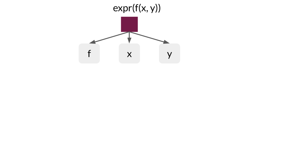

---
![Source: modified from Hadley Wickham's Tidy evaluation in 5 mins](images/unquoting_tree_1.png)

---
![Source: modified from Hadley Wickham's Tidy evaluation in 5 mins](images/unquoting_tree_2.png)

---
## `!!` inserts the code tree sorted into the expression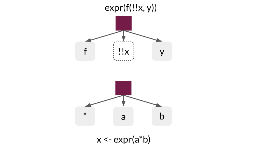
![Source: modified from Hadley Wickham's Tidy evaluation in 5 mins](images/unquoting_tree_3.png)

---
![Source: modified from Hadley Wickham's Tidy evaluation in 5 mins](images/unquoting_tree_4.png)

---
## Unquoting makes it easy to build trees
![Source: modified from Hadley Wickham's Tidy evaluation in 5 mins](images/unquoting_tree_5.png)

---
# 3. code can generate code
<img src="images/unquoting_tree_5.png" width="400px" />

In code it would look like this.

```r
x <- expr(a*b)
expr(f(!!x, y))
#> f(a * b, y)
```

---
# 3. code can generate code
In the book there is also this example:

```r
xx <- expr(x + x)
yy <- expr(y + y)

expr(!!xx / !!yy)
#> (x + x)/(y + y)
```
What's really nice in this example is that the _order of the expression_ is maintained, and brackets are added automatically.

---
# 3. code can generate code
gets even more useful if you wrap it up into a function, first using `enexpr()` to capture the users expression then `expr()` and `!!` to create a new expression using a template.

```r
cv <- function(var) {
  var <- enexpr(var)
  expr(sd(!!var) / mean(!!var))
}

cv(x)
#> sd(x)/mean(x)
cv(x + y)
#> sd(x + y)/mean(x + y)
```

---
# 4. evaluation runs code
We looked at a lot of captured code and expressions, next up is the **evaluation** of an expression. Evaluating an expression requires an environment.
--

`base::eval()` can be used. Here you can specify the expression and the environment:

```r
eval(expr(x + y), env(x = 1, y = 10))
#> [1] 11
eval(expr(x + y), env(x = 2, y = 100))
#> [1] 102
```
--

If `env()` is not specified, it uses the current environment:

```r
x <- 10
y <- 100
eval(expr(x + y))
#> [1] 110
```
--

_Why tweaking the environment?_
- allows to temporarily override functions to implement a domain specific language
- to add a data mask so you can refer to variables in a dataframe as if they are variables in an environment (Tip: tidyverse ;))

---
# summary- what you know by now (2)
- **metaprogramming** = programming the program
- code is data, you can capture code (once captured = **expression**). Can be inspected and manipulated on as you can with any type of data. In `R`, code can be captured with `expr()` or `enexpr()`. 
- code is organised in a tree. This allows to explore `R`'s grammar through inspection and manipulation. In `R` you can observe the tree with `lobstr::ast()`
--

- Code can generate code: to do so we can use `expr()` and `enexpr()` with  `!!` (bang-bang), the unquoting operator.
--

- To run code it has to be **evaluated** within the current or a specified environment. In `R` you can do this with the `base::eval()` function.
--

### Are we still good? Questions?

---
#5. customising evaluation with functions
- previously we bound `x` and `y` to vectors
- it's less obvious, but you can also bind names to functions, allowing to override behavior of existing functions.
--

- For example, you can override the function of `+` and `*` to work with strings instead of numbers.

```r
string_math <- function(x) {
  e <- env(
    caller_env(),
    `+` = function(x, y) paste0(x, y),
    `*` = function(x, y) strrep(x, y)
  )

eval(enexpr(x), e)
}

name <- "Hadley"
string_math("Hello " + name)
#> [1] "Hello Hadley"
string_math(("x" * 2 + "-y") * 3)
#> [1] "xx-yxx-yxx-y"
```

`dplyr` takes this idea to the extreme, running code in an environment that generates `SQL` for execution in a remote database.

---
# 6. customising evaluation with data
- idea to modify evaluations to look for variables in a dataframe as if it was an environment.
--

- Idea underlying many tidyverse functions e.g. `ggplot2::aes()` or `dplyr::mutate()`
--

- if data frame temporarily masks the workspace, we talk of **data masks**, data masks are only possible because `R` allows to suspend the normal flow of evaluation
- **data mask**- enable to pass on dataframes instead of environments to be evaluated used with`eval_tidy()`
--

```r
df <- data.frame(x = 1:5, y = sample(5))
rlang::eval_tidy(expr(x + y), df)
#> [1] 2 6 5 9 8
```

useful, as it allows you to write `x+y` instead of `df$x + df$y`

---
# 6. customising evaluation with data
Let's assume we have this function

```r
with2 <- function(df, expr) {
  a <- 1000
  eval_tidy(enexpr(expr), df)
}
```
--

```r
df <- data.frame(x = 1:3)
a <- 10
with2(df, x + a)
#> [1] 1001 1002 1003
```

if we use a variable from the outside called `a`, we want this variable (10) to be used if we passed it in as an argument. But the function will take the `a` that has been specified within the function.

---
# 7. quosures
- a new data structure can solve the issue we just saw
- **Quosures** - bundles an expression with an environment

```r
quo(x)
#> <quosure>
#> expr: ^x
#> env:  global
```
- a quosure consists of two parts. the `expr` - expression and the `env`- environment, they are objects and so can be passed around, carrying their environment with them
- `enquo()` needed to capture the correct environment
--

- to fix the above problem, all we have to do is to replace `enexpr()` with `enquo()`

```r
with2 <- function(df, expr) {
  a <- 1000
  eval_tidy(enquo(expr), df)
}

with2(df, x + a)
#> [1] 11 12 13
```

---
# Summary- what you know by now (3)
- **metaprogramming** = programming the program
- code is data, you can capture code (once captured = **expression**). Can be inspected and manipulated on as you can with any type of data. In `R`, code can be captured with `expr()` or `enexpr()`. 
- code is organised in a tree. This allows to explore `R`'s grammar through inspection and manipulation. In `R` you can observe the tree with `lobstr::ast()`
- Code can generate code: to do so we can use `expr()` and `enexpr()` with  `!!` (bang-bang), the unquoting operator.
- To run code it has to be **evaluated** within the current or a specified environment. In `R` you can do this with the `base::eval()` function.
--

- Customising evaluation with functions, complex, but useful for `dbplyr` for example
--

- Customising evaluation with data: **data masks** enable to pass on dataframes instead of environments to be evaluated, In `R` you can do this with `eval_tidy()`.
--

- **Quosures**- new data structure that bundles an expression and an environment together.

---
## So what's the solution for `plot_scatter()`?

As you might recall we had this function

```r
ggplot(starwars, 
       aes(mass, height)) +
geom_point()
```
--

that we wanted to rewrite into:

```r
plot_scatter <- function(data, x_col, y_col) {
  ggplot(data, # normal r rules
       aes(x_col, y_col)) + # special r rules
geom_point()
}
```

---
calling it on mtcars resulted in several errors.

```r
plot_scatter(mtcars, disp, mpg)
#> Error in FUN(X[[i]], ...) : object 'disp' not found

plot_scatter(mtcars, 'disp', 'mpg')
#> Error in FUN(X[[i]], ...) : object 'disp' not found

plot_scatter(mtcars, mtcars$disp, mtcars$mpg)
#> Error: Aesthetics must be either length 1 or the same as the data (87): x and y
```

---

```r
plot_scatter <- function(data, x_col, y_col) {
  ggplot(data, # normal r rules
       aes(x_col, y_col)) + # special r rules
geom_point()
}
```

The function has to be modyfied with arguments we just learned about.
1) we need to identify all arguments where the user refers to the dataframe columns directly, such that it can _not_ be evaluated right away
--

```r
plot_scatter <- function(data, x_col, y_col) {
  x_col <- enquo(x_col)
  y_col <- enquo(y_col)
  ggplot(data, # normal r rules
       aes(x_col, y_col)) + # special r rules
geom_point()
}
```
--

2) Identify where these variables are passed to other quoting functions
--

```r
plot_scatter <- function(data, x_col, y_col) {
  x_col <- enquo(x_col)
  y_col <- enquo(y_col)
  ggplot(data, # normal r rules
       aes(!!x_col, !!y_col)) + # special r rules
geom_point()
}
```

---
Let's try it with mtcars

```r
plot_scatter(mtcars, disp, mpg)
```

We end up with a function that automatically quotes and unquotes the function where needed. :)

---
# What's next?

- Can't get enough?
- join the upcoming bookclub sessions for a deepdive
- reread Chapter 17 :)
- Read about [tidyeval](https://tidyeval.tidyverse.org/)
- [Hadley capturing the main ideas in 5 mins](https://www.youtube.com/watch?v=nERXS3ssntw)

---
# Thanks to:

- Hadley Wickham for writing [AdvancedR](https://adv-r.hadley.nz/)
- R Core Team (2020). R: A language and environment for statistical computing. R Foundation for Statistical Computing,
  Vienna, Austria. [URL](https://www.R-project.org/).  
- Yihui Xie (2020). [xaringan](https://CRAN.R-project.org/package=xaringan): Presentation Ninja. R package version 0.16. 
- Garrick Aden-Buie (2020). [xaringanExtra](https://github.com/gadenbuie/xaringanExtra): Extras And Extensions for Xaringan Slides. R package version 0.0.17.

and all the authors of R packages used in this presentation

---

# Thank you and see you in two weeks!
--

![](https://media.giphy.com/media/3oEdva9BUHPIs2SkGk/giphy.gif)
---